[MLB 스탯캐스트] 머신러닝으로 MLB 타자들의 최종 홈런 성적 예측해보기 - 1. EDA & Data Engineering

머신러닝 코드 및 데이터자료 (아래 링크의 Predict_HR 폴더)

https://github.com/JeongMinHyeok/Handling_MLB_Statcast

GitHub - JeongMinHyeok/Handling_MLB_Statcast

 

데이터셋 출처 :

https://baseballsavant.mlb.com/

Baseball Savant: Trending MLB Players, Statcast and Visualizations

---

MLB 전반기가 끝나고 올스타전이 열리면서, 잠시동안 MLB도 휴식기를 가지게 되었다.

원래 계획은 이 올스타 휴식기에 이 프로젝트를 해보려고 했지만... 좀 늦어졌다.

 

이번에는 머신러닝을 통해서 타자들의 최종 홈런 성적을 예상해보려고 한다.

MLB Statcast에서 제공하는 여러 정보들을 가지고, 머신러닝의 앙상블 모델을 활용해 예측을 할 계획이다.

 

타자들의 이름과 id, 여러 지표들 등 39개의 칼럼에 해당하는 특징이 있는 데이터셋을 다운로드 받았으며,

훈련 데이터로는 스탯캐스트 지표가 제공되는 2015년부터 2019년까지의 데이터,

(2020년은 단축 시즌이기때문에, 데이터셋에서 제외했다.)

검증 데이터로는 2021년 현재 (7월 22일)의 데이터를 사용했다.

 

 

데이터셋에 포함된 칼럼

• 'last_name'
• 'first_name'
• 'player_id'
• 'year'
• 'b_ab'
• 'b_total_pa'
• 'b_home_run'
• 'batting_avg'
• 'slg_percent'
• 'on_base_percent',
• 'on_base_plus_slg'
• 'xba'
• 'xslg'
• 'woba'
• 'xwoba'
• 'xobp'
• 'xiso'
• 'wobacon'
• 'xwobacon'
• 'bacon'
• 'xbacon'
• 'xbadiff'
• 'xslgdiff',
• 'wobadif'
• 'exit_velocity_avg'
• 'launch_angle_avg',
• 'sweet_spot_percent'
• 'barrels'
• 'barrel_batted_rate',
• 'poorlyweak_percent'
• 'hard_hit_percent'
• 'z_swing_percent',
• 'z_swing_miss_percent'
• 'oz_swing_miss_percent'
• 'oz_contact_percent',
• 'groundballs_percent'
• 'flyballs_percent'
• 'linedrives_percent'

---

EDA & Feature Engineering

# 2015 ~ 2020 데이터 살펴보기
df_old.head()

print(df_old.shape)
print(df_now.shape)

>>>
(850, 39)
(137, 40)

데이터셋은 위와 같은 모습이다.

 

 

필요없는 칼럼 삭제

• 선수이름, Unnamed:(?) 칼럼 삭제
• 2020년 데이터 삭제 (단축시즌이었기 때문에)
• 연도표시 칼럼 삭제
• 2021년 데이터의 player_id, 이름은 따로 저장 (예측때 사용)

# 선수이름, Unamed 칼럼 삭제
df_old = df_old.drop(['last_name', ' first_name', 'Unnamed: 38'], axis=1)
player_id = df_now['player_id']
name = df_now['last_name'] + df_now[' first_name']
df_now = df_now.drop(['last_name', ' first_name', 'Unnamed: 39'], axis=1)

# 2020년 데이터 삭제
df_old = df_old[df_old.year != 2020]

# 연도 칼럼 삭제
df_old = df_old.drop(['year'], axis=1)
df_now = df_now.drop(['year'], axis=1)

 

상관관계 분석

- 홈런갯수와 칼럼들 사이의 상관관계를 분석해보았다.

# 상관계수가 0.4이상인 칼럼들 나타내기

corr = df_old.corr()
corr_columns = corr.index[abs(corr['b_home_run']) >= 0.4]
corr_columns

>>>
Index(['b_home_run', 'slg_percent', 'on_base_plus_slg', 'xslg', 'woba',
       'xwoba', 'xobp', 'xiso', 'wobacon', 'xwobacon', 'xbacon',
       'exit_velocity_avg', 'launch_angle_avg', 'barrels',
       'barrel_batted_rate', 'hard_hit_percent', 'z_swing_miss_percent',
       'groundballs_percent', 'flyballs_percent'],
      dtype='object')

# heatmap

plt.figure(figsize=(13,10))
heatmap = sns.heatmap(df_old[corr_columns].corr(),annot=True,cmap="RdYlGn")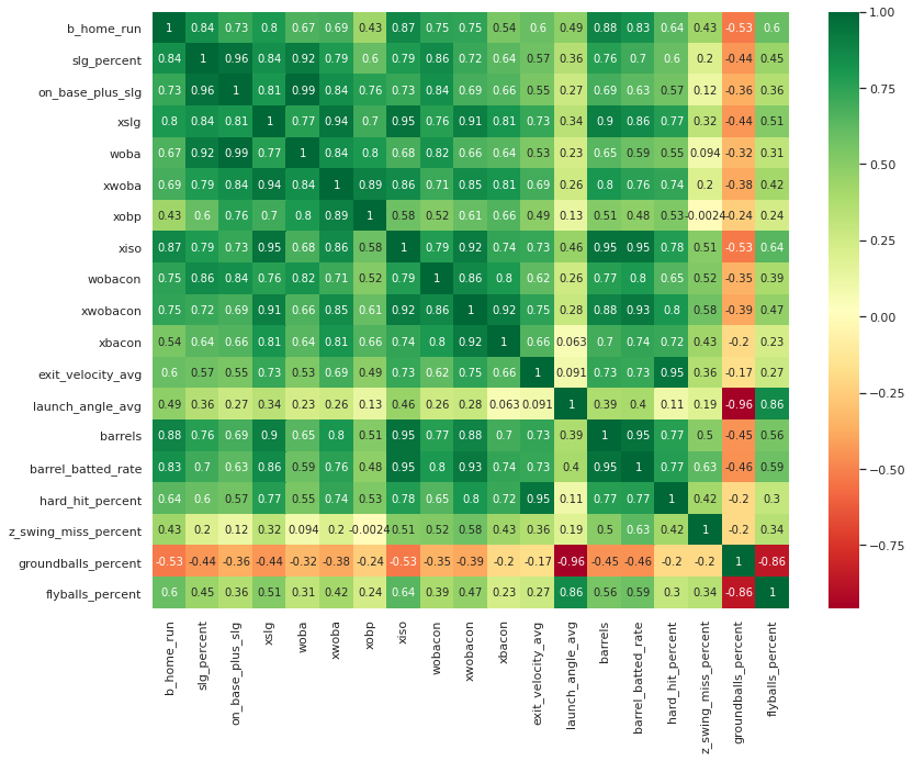

• 다중공산성이 매우 높아 문제를 일으킬 가능성 높음

 

VIF (Variance Inflation Factor) 사용

• 다른 독립변수에 의존하는(VIF가 높은) 변수 삭제
• VIF 수치가 높은 칼럼들을 삭제해가면서, VIF가 변하는 모습 살펴보기
• 충분히 수치가 낮아지면 해당 칼럼들 사용

vif_old = df_old.drop(['groundballs_percent', 'oz_swing_miss_percent', 'z_swing_percent', 'z_swing_percent', 'batting_avg', 'slg_percent', 'on_base_percent', 'woba', 'wobacon', 'on_base_plus_slg', 'bacon'], axis=1)

from statsmodels.stats.outliers_influence import variance_inflation_factor

vif = pd.DataFrame()
vif["VIF Factor"] = [float(variance_inflation_factor(
    vif_old.values, i)) for i in range(vif_old.shape[1])]
vif["features"] = vif_old.columns
vif.sort_values('VIF Factor')
vif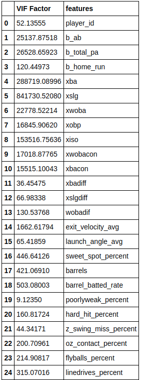

# 확정
df_old = df_old.drop(['groundballs_percent', 'oz_swing_miss_percent', 'z_swing_percent', 'z_swing_percent', 'batting_avg', 'slg_percent', 'on_base_percent', 'woba', 'wobacon', 'on_base_plus_slg', 'bacon'], axis=1)

 

칼럼 하나씩 살펴보고 이상치 제거 / 제외할 칼럼 선정 (Outlier remove)

• 분석 대상 :
  • 'xba', 'xslg', 'xwoba', 'xobp', 'xiso', 'xwobacon', 'xbacon', 'xbadiff', 'xslgdiff', 'wobadif', 'exit_velocity_avg', 'launch_angle_avg', 'sweet_spot_percent', 'barrels', 'barrel_batted_rate', 'poorlyweak_percent', 'hard_hit_percent' 'z_swing_miss_percent', 'oz_contact_percent', 'flyballs_percent', 'linedrives_percent'
• 주요 칼럼들만 분석 소개

xBA - 기대타율

• 타율은 생각보다 홈런과 큰 관계없음

xISO - 기대 순수장타율 (장타율 - 타율)

• 강한 상관관계 보임

xWOBACON - 기대가중출루율 (컨택된 타구에 대한)

• 압도적인 xWOBACON의 2017시즌 아론 저지(0.640 정도)... 학습에 영향줄 수 있으므로 삭제

추가 제외할 칼럼 선정

• xba / xbadiff / xslgdiff / wobadif / sweet_spot_percent / poorlyweak_percent / linedirves_percent
• 산점도 분석을 통해 상관관계가 비교적 적고, 학습에 영향을 줄만한 칼럼들 삭제
• test data에도 같은 칼럼을 가지도록 삭제

df_old = df_old.drop(['xba', 'xbadiff', 'xslgdiff', 'wobadif', 'sweet_spot_percent', 'poorlyweak_percent', 'linedrives_percent'], axis=1)

df_now = df_now.drop(['groundballs_percent', 'oz_swing_miss_percent', 'z_swing_percent', 'z_swing_percent', 'batting_avg', 'slg_percent', 'on_base_percent', 'woba', 'wobacon', 'on_base_plus_slg', 'bacon', 'xba', 'xbadiff', 'xslgdiff', 'wobadif', 'sweet_spot_percent', 'poorlyweak_percent', 'linedrives_percent'], axis=1)

 

현재 데이터에 부족한 게임 수 조정하기

• 메이저리그 총 경기 168경기에 현재 출전경기비율 계산 (전 경기 출장했다고 가정)
• 출전경기비율을 타석과 배럴타구 수(barrels)에 168경기 기준으로 계산되도록 위의 비율을 통해 조정

df_now['progress'] = df_now['b_game'] / 168
df_now['progress'] = df_now['progress'] + 1

df_now['b_ab'] = round(df_now['b_ab'] * df_now['progress'], 0)
df_now['b_total_pa'] = round(df_now['b_total_pa'] * df_now['progress'], 0)
df_now['barrels'] = round(df_now['barrels'] * df_now['progress'], 0)

 

target (홈런개수) 살펴보기

• 그래프를 통해 편향성 알아보기
• 양의 왜도값을 가짐
• log변환을 통해 정규성을 띄도록 변환한 값 확인

import matplotlib.pyplot as plt
import seaborn as sns
sns.set()
%matplotlib inline

sns.distplot(df_old['b_home_run'])

• 로그변환

# old data에서 로그변환한 홈런 칼럼 따로 저장하고 삭제
y_data = np.log1p(df_old['b_home_run'])
df_old = df_old.drop(['b_home_run'], axis=1)

 

EDA와 Data Handling에 이어 다음 게시물에는 학습모델링 과정을 설명하고,

예측 결과까지 설명해보겠다.